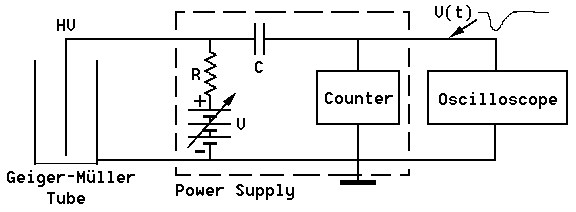
Figure 1: Geiger-Müller apparatus and connection diagram
| PHY 252 | Geiger Counter |
This experiment has two main objectives. First, we will become familiar with the characteristics of the Geiger-Müller (GM) tube, including the properties of threshold, starting and operating voltages, GM plateau region and plateau slope. Then we will use the GM tube to perform a simple statistical experiment for the purpose of studying some of the techniques of statistical analysis.
The basic GM circuit diagram is shown in Figure 1. The power supply and counter are one unit. The GM tube itself consists of a cylindrical outer shell which serves as a cathode and is grounded. In the center it has a coaxially mounted wire serving as anode. The cylinder is filled with an inert gas (typically Argon) at low pressure plus a small amount of ``quenching'' gas (e.g. ethyl alcohol).
A DC power supply provides a voltage across the tube in the range of a few hundred to over a thousand Volts depending on the requirements of the particular tube. Caution: The front window of the tube is very thin and delicate and should not be touched.

Figure 1: Geiger-Müller apparatus and connection diagram
Radiation entering the tube can ionize some of the gas atoms, thereby freeing electrons which are accelerated towards the central wire by the electric field and gaining enough energy to cause further ionization. The result is a ``cascade'' or ``avalanche'' effect which produces a current pulse through the tube. This current pulse causes a voltage pulse across resistor R, which is used to trigger a counting device that records the number of pulses. We are thus able to count the number of ionizing particles entering the tube. There is, however, no information about the initial particle energy. An oscilloscope is connected to the system to allow us to visually observe the pulses from the tube.
The purpose of the quenching additive to the gas is to effectively absorb UV-photons emitted from the electrodes when the ions produced in the multiplication process impact on the electrodes. Such photons may otherwise liberate secondary electrons (via the photo-electric effect) which may initiate the avalanche process all over again, thereby leading to catastrophic breakdown of the tube (i.e. a spark).
 |
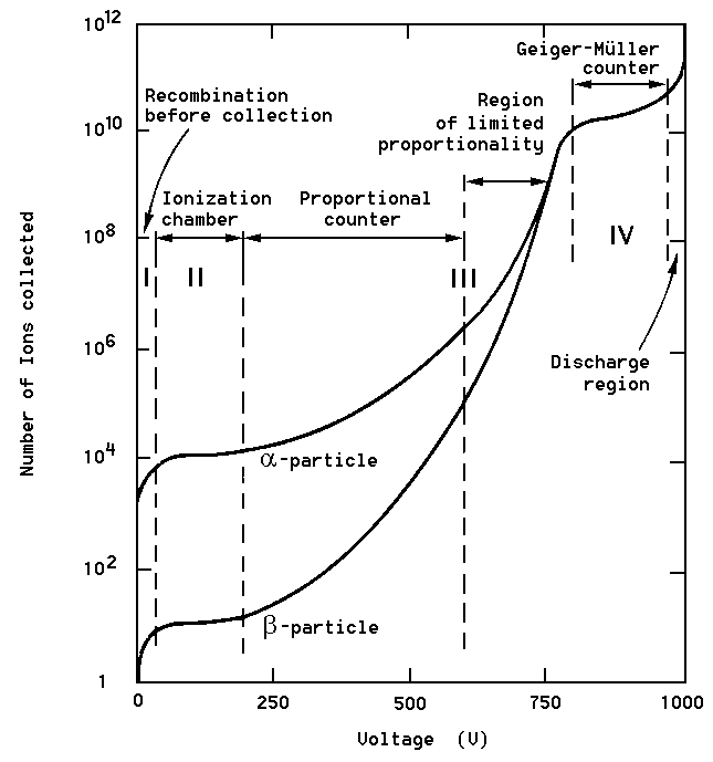
Figure 2: The number of electron-ion pairs collected when a charged particle traverses a gaseous counter of average size, plotted against the voltage applied between electrodes. The curves are for a-particles (He nuclei) and b-particles (electrons). Note the three regions of operation as an (I) ionization counter, (II) proportional counter, and (IV) Geiger-Müller counter. |
Determine the mean number of counts <N> and the standard deviation s. The result should approximate the ``Poisson'' distribution, for which the probability P for observing N counts in a given time interval is given by
P(N) = <N>N e-<N> / N! , s = Ö<N> .
Compare your graph with this expression. Also, compare your results with the Figure shown here.