|
Undergraduate Physics |
Error Analysis |
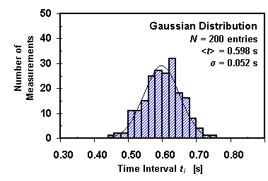
Every measurement an experimenter makes is uncertain to some degree. The uncertainties are of two kinds: (1) random errors, or (2) systematic errors. For example, in measuring the time required for a weight to fall to the floor, a random error will occur when an experimenter attempts to push a button that starts a timer simultaneously with the release of the weight. If this random error dominates the fall time measurement, then if we repeat the measurement many times (N times) and plot equal intervals (bins) of the fall time ti on the horizontal axis against the number of times a given fall time ti occurs on the vertical axis, our results (see histogram below) should approach an ideal bell-shaped curve (called a Gaussian distribution) as the number of measurements N becomes very large.

The best estimate of the true fall time t is the mean value (or average value) of the distribution:
átñ = (SNi=1 ti)/N .
If the experimenter squares each deviation from the mean, averages the squares, and takes the square root of that average, the result is a quantity called the "root-mean-square" or the "standard deviation" s of the distribution. It measures the random error or the statistical uncertainty of the individual measurement ti:
s
= Ö[SNi=1(ti - átñ)2 / (N-1) ].About two-thirds of all the measurements have a deviation less than one s from the mean and 95% of all measurements are within two s of the mean. In accord with our intuition that the uncertainty of the mean should be smaller than the uncertainty of any single measurement, measurement theory shows that in the case of random errors the standard deviation of the mean smean is given by:
s
m = s / ÖN ,where N again is the number of measurements used to determine the mean. Then the result of the N measurements of the fall time would be quoted as t = átñ ± sm.
Whenever you make a measurement that is repeated N times, you are supposed to calculate the mean value and its standard deviation as just described. For a large number of measurements this procedure is somewhat tedious. If you have a calculator with statistical functions it may do the job for you. There is also a simplified prescription for estimating the random error which you can use. Assume you have measured the fall time about ten times. In this case it is reasonable to assume that the largest measurement tmax is approximately +2s from the mean, and the smallest tmin is -2s from the mean. Hence:
s
» ¼ (tmax - tmin)is an reasonable estimate of the uncertainty in a single measurement. The above method of determining s is a rule of thumb if you make of order ten individual measurements (i.e. more than 4 and less than 20).
Not all errors are statistical in nature. That means some measurements cannot be improved by repeating them many times. For example, assume you are supposed to measure the length of an object (or the weight of an object). The accuracy will be given by the spacing of the tickmarks on the measurement apparatus (the meter stick). You can read off whether the length of the object lines up with a tickmark or falls in between two tickmarks, but you could not determine the value to a precision of l/10 of a tickmark distance. Typically, the error of such a measurement is equal to one half of the smallest subdivision given on the measuring device. So, if you have a meter stick with tickmarks every mm (millimeter), you can measure a length with it to an accuracy of about 0.5 mm. While in principle you could repeat the measurement numerous times, this would not improve the accuracy of your measurement!
Note: This assumes of course that you have not been sloppy in your measurement but made a careful attempt to line up one end of the object with the zero of the meter stick as accurately as you can, and that you read off the other end of the meter stick with the same care. If you want to judge how careful you have been, it would be useful to ask your lab partner to make the same measurements, using the same meter stick, and then compare the results.
Systematic errors result when characteristics of the system we are examining, or the instruments we use are different from what we assume them to be. For example, if a voltmeter we are using was calibrated incorrectly and reads 5% higher than it should, then every voltage reading we record using this meter will have an error of 5%. Clearly, taking the average of many readings will not help us to reduce the size of this systematic error. If we knew the size and direction of the systematic error we could correct for it and thus eliminate its effects completely. Even when we are unsure about the effects of a systematic error we can sometimes estimate its size (though not its direction) from knowledge of the quality of the instrument. For example, the meter manufacturer may guarantee that the calibration is correct to within 1%. (Of course, one pays more for an instrument that is guaranteed to have a small error.)
Even simple experiments usually call for the measurement of more than one quantity. The experimenter inserts these measured values into a formula to compute a desired result. He/she will want to know the uncertainty of the result. Here, we list several common situations in which error propagion is simple, and at the end we indicate the general procedure. If you are faced with a complex situation, ask your lab instructor for help.
Many types of measurements, whether statistical or systematic in nature, are not distributed according to a Gaussian. Examples are the age distribution in a population, and many others. However, it can be shown that if a result R depends on many variables, than evaluations of R will be distributed rather like a Gaussian - and more so when R depends on more variables - , even when the individual variables are not. The theorem In the following, we assume that our measurements are distributed as simple Gaussians.
When a result R is calculated from two measurements x and y, with uncertainties Dx and Dy, and two constants a and b with the additive formula:
R = ax + by ,
and if the errors in x and y are independent, then the error in the result R will be:
(D
R)2 = (a Dx)2 + (b Dy)2 .The reason why we should use this quadratic form and not simply add the uncertainties aDx and bDy, is that we don't know whether x and y were both measured too large or too small; indeed the measurement errors on x and y might cancel each other in the result R! Independent errors cancel each other with some probability (say you have measured x somewhat too big and y somewhat too small; the error in R might be small in this case). This partial statistical cancellation is correctly accounted for by adding the uncertainties quadratically.
Note: a and b can be positive or negative, i.e. the equation works for both addition and subtraction.
When the result R is calculated by multiplying a constant a times a measurement of x times a measurement of y (or divided by y), i.e.:
R = axy or R = ax/y,
then the relative errors Dx/x and Dy/y add quadratically:
(DR/R)2 = (Dx/x)2 + (Dy/y)2 .
Example: Say quantity x is measured to be 1.00, with an uncertainty Dx = 0.10, and quantity y is measured to be 1.50 with uncertainty Dy = 0.30, and the constant a = 5.00 . The result R is obtained as R = 5.00 ´ 1.00 ´ l.50 = 7.5 . The relative uncertainty in x is Dx/x = 0.10 or 10%, whereas the relative uncertainty in y is Dy/y = 0.20 or 20%. Therefore the relative error in the result is DR/R = Ö(0.102 + 0.202) = 0.22 or 22%,. The absolute uncertainty of the result R is obtained by multiplying 0.22 with the value of R: DR = 0.22 ´ 7.50 = 1.7 .
If your result is obtained using a more complicated formula, as for example:
R = a x2 siny ,
there is a very easy way to find out how your result R is affected by errors Dx and Dy in x and y. Insert into the equation for R, instead of the value of x, the value x+Dx, and find how much R changes:
R + DRx = a (x+Dx)2 siny .
If y has no error you are done. If y has an error as well, do the same as you just did for x, i.e. insert into the equation for R the value for y+Dy instead of y, to obtain the error contribution DRy. The total error of the result R is again obtained by adding the errors due to x and y quadratically:
(DR)2 = (DRx)2 + (DRy)2 .
This way to determine the error always works and you could use it also for simple additive or multiplicative formulae as discussed earlier. Also, if the result R depends on yet another variable z, simply extend the formulae above with a third term dependent on Dz.
The above formulae are in reality just an application of the Taylor series expansion: the expression of a function R at a certain point x+Dx in terms of its value and derivatives in a neighboring point x. For the error estimates we keep only the first terms:
DR = R(x+Dx) - R(x) = (dR/dx)x Dx for Dx ``small'',
where (dR/dx)x is the derivative of function R with respect to variable x, evaluated at point x. As before, when R is a function of more than one uncorrelated variables (x, y, z, ...), take the total uncertainty as the square root of the sum of individual squared uncertainties:
(DR)2 = (Dx (dR/dx)x)2 + (Dy (dR/dy)y)2 + (Dz (dR/dz)z)2 + ...
where, in the above formula, we take the derivatives dR/dx etc. to be partial derivatives.
In light of the above discussion of error analysis, discussions of significant figures (which you should have had in previous courses) can be seen to simply imply that an experimenter should quote digits which are appropriate to the uncertainty in his result. The above result of R = 7.5 ± 1.7 illustrates this. It would not be meaningful to quote R as 7.53142 since the error affects already the first figure. On the other hand, to state that R = 8 ± 2 is somewhat too casual. It is a good rule to give one more significant figure after the first figure affected by the error.
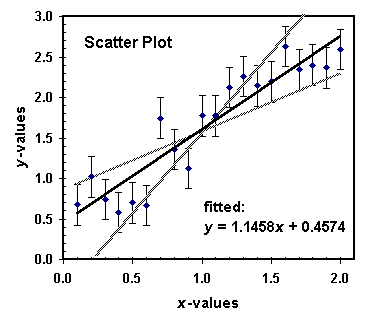
Frequently in the laboratory you will have the situation that you perform a series of measurements of a quantity y at different values of x, and when you plot the measured values of y versus x you observe a linear relationship of the type y = ax + b. Your task is now to determine, from the errors in x and y, the uncertainty in the measured slope a and the intercept b. There is a mathematical procedure to do this, called "linear regression" or "least-squares fit". Such fits are typically implemented in spreadsheet programs and can be quite sophisticated, allowing for individually different uncertainties of the data points and for fits of polynomials, exponentials, Gaussian, and other types of functions to the data. If you have no access or experience with spreadsheet programs, you want to instead use a simple, graphical method, briefly described in the following.
Plot the measured points (x,y) and mark for each point the errors Dx and Dy as bars that extend from the plotted point in the x and y directions. Draw the line that best describes the measured points (i.e. the line that minimizes the sum of the squared distances from the line to the points to be fitted; the least-squares line). This line will give you the best value for slope a and intercept b. Next, draw the steepest and flattest straight lines, see the Figure, still consistent with the measured error bars. From these two lines you can obtain the largest and smallest values of a and b still consistent with the data, amin and bmin, amax and bmax. From their deviation from the best values you then determine, as indicated in the beginning, the uncertainties Da and Db.
